Model: Regressing binary dependent variable, DRINKING_D, on the following binary and continuous predictors: FATAL_OR_M, OVERTURNED, CELL_PHONE, SPEEDING, AGGRESSIVE, DRIVER1617, DRIVER65PLUS, PCTBACHMOR, and MEDHHINC.
Prior to running any of the analyses, be sure to set the working directory using the setwd command, install the relevant R packages using the install.packages command, and load the relevant packages using the library command.
# 4. Generate the kable tabledrink_table <-kbl(drink_summary_df,caption ="Summary of Alcohol Consumption",align ="c",escape =FALSE ) %>%kable_styling(bootstrap_options ="striped",full_width = F ) %>%row_spec(0, bold = T)drink_table
Summary of Alcohol Consumption
Metric
No Alcohol
Alcohol
Count
40,879
2,485
Proportion
0.94
0.06
Code
# Save as HTML file.#save_kable(drink_table, "drink_table.html", zoom = 3, self_contained = TRUE)# Then convert HTML to PNG using webshot.#webshot::webshot("drink_table.html", "drink_table.png")
In your report, in addition to the counts that you can obtain with the table command, you will be asked to report the proportion of crashes that involved a drunk driver using the prop.table command as above.
2.b. Using the CrossTable command in the gmodels library, examine the cross-tabulations between the dependent variable, DRINKING_D, and the following binary predictor variables: FATAL_OR_M, OVERTURNED, CELL_PHONE, SPEEDING, AGGRESSIVE, DRIVER1617, and DRIVER65PLUS.
2.b.i. For the first predictor (FATAL_OR_M), record the number and percentage of 1-responses (i.e., fatalities or major injuries) for both categories of the variable DRINKING_D, as well as the total number of 1-responses (i.e., fatalities or major injuries) in the data set. That is, how many fatalities or major injuries were there when the driver wasn’t inebriated, when the driver was inebriated, and altogether?
2.b.ii. Repeat step 2.b.i above for the rest of the binary predictors.
Code
# I made a function to loop through it so I don't have to do this 7 separate times.# Create predictor vector.predictors <-c("FATAL_OR_M", "OVERTURNED", "CELL_PHONE","SPEEDING", "AGGRESSIVE","DRIVER1617", "DRIVER65PLUS" )# Create an empty results dataframe.binary_results <-data.frame(Predictor =character(),Drink0_Count_1 =numeric(),Drink1_Count_1 =numeric(),Total_1 =numeric(),ChiSq =numeric(),p_value =numeric(),stringsAsFactors =FALSE)# Loop through each predictor.for (var in predictors) {cat("=======================================================\n")cat("PREDICTOR:", var, "\n")# Build 2x2 table. tab <-table(cdc_data$DRINKING_D, cdc_data[[var]])print(tab)# Row percentages.cat("\nRow percentages (within DRINKING_D):\n")print(round(prop.table(tab, 1), 4))# Count the number of 1's. total_ones <-sum(cdc_data[[var]] ==1)cat("\nTotal number of", var, "= 1 in dataset:", total_ones, "\n")# Chi-square test. test <-chisq.test(tab, correct =FALSE)cat("\nChi-square statistic:", test$statistic,"\nDegrees of freedom:", test$parameter,"\np-value:", test$p.value, "\n")# Add row to results dataframe. binary_results <-rbind( binary_results,data.frame(Predictor = var,Drink0_Count_1 = tab["0", "1"],Drink1_Count_1 = tab["1", "1"],Total_1 = total_ones,ChiSq =unname(test$statistic),p_value = test$p.value ) )}
=======================================================
PREDICTOR: FATAL_OR_M

        0     1
  0 39698  1181
  1  2297   188

Row percentages (within DRINKING_D):

         0      1
  0 0.9711 0.0289
  1 0.9243 0.0757

Total number of FATAL_OR_M = 1 in dataset: 1369

Chi-square statistic: 167.5615
Degrees of freedom: 1
p-value: 0.00000000000000000000000000000000000002522202
=======================================================
PREDICTOR: OVERTURNED

        0     1
  0 40267   612
  1  2375   110

Row percentages (within DRINKING_D):

         0      1
  0 0.9850 0.0150
  1 0.9557 0.0443

Total number of OVERTURNED = 1 in dataset: 722

Chi-square statistic: 122.788
Degrees of freedom: 1
p-value: 0.0000000000000000000000000001551762
=======================================================
PREDICTOR: CELL_PHONE

        0     1
  0 40453   426
  1  2457    28

Row percentages (within DRINKING_D):

         0      1
  0 0.9896 0.0104
  1 0.9887 0.0113

Total number of CELL_PHONE = 1 in dataset: 454

Chi-square statistic: 0.162071
Degrees of freedom: 1
p-value: 0.6872569
=======================================================
PREDICTOR: SPEEDING

        0     1
  0 39618  1261
  1  2225   260

Row percentages (within DRINKING_D):

         0      1
  0 0.9692 0.0308
  1 0.8954 0.1046

Total number of SPEEDING = 1 in dataset: 1521

Chi-square statistic: 376.7808
Degrees of freedom: 1
p-value: 0.000000000000000000000000000000000000000000000000000000000000000000000000000000000006249562
=======================================================
PREDICTOR: AGGRESSIVE

        0     1
  0 22357 18522
  1  1569   916

Row percentages (within DRINKING_D):

         0      1
  0 0.5469 0.4531
  1 0.6314 0.3686

Total number of AGGRESSIVE = 1 in dataset: 19438

Chi-square statistic: 67.60186
Degrees of freedom: 1
p-value: 0.000000000000000200079
=======================================================
PREDICTOR: DRIVER1617

        0     1
  0 40205   674
  1  2473    12

Row percentages (within DRINKING_D):

         0      1
  0 0.9835 0.0165
  1 0.9952 0.0048

Total number of DRIVER1617 = 1 in dataset: 686

Chi-square statistic: 20.45167
Degrees of freedom: 1
p-value: 0.000006115619
=======================================================
PREDICTOR: DRIVER65PLUS

        0     1
  0 36642  4237
  1  2366   119

Row percentages (within DRINKING_D):

         0      1
  0 0.8964 0.1036
  1 0.9521 0.0479

Total number of DRIVER65PLUS = 1 in dataset: 4356

Chi-square statistic: 80.6047
Degrees of freedom: 1
p-value: 0.000000000000000000275703
2.b.iii. In your report, you will be asked to present the cross-tabulations from 2.b.i and 2.b.ii in a table.
2.b.iv. Prior to doing predictive modeling, statisticians often use the Chi-Square (χ2) test to determine whether the distribution of one categorical variable varies with respect to the values of another categorical variable. If we were to look at a cross-tabulation of the variables DRINKING_D and FATAL_OR_M, the null and alternative hypotheses for the χ2 test would be as follows:
H0: The proportion of fatalities for crashes that involve drunk drivers is the same as the proportion of fatalities for crashes that don’t involve drunk drivers.
vs.
Ha: The proportion of fatalities for crashes that involve drunk drivers is different than the proportion of fatalities for crashes that don’t involve drunk drivers.
As usual, a high value of the χ2 statistic, and a p-value lower than 0.05 suggest that there’s evidence to reject the null hypothesis in favor of the alternative, and that there’s an association between drunk driving and crash fatalities.
2.b.iv.1. To carry out the χ2 test in R to test the hypothesis above, you would use the syntax CrossTable(cdc_data$FATAL_OR_M, cdc_data$DRINKING_D, prop.r = FALSE, prop.t = FALSE, prop.chisq = FALSE, chisq = TRUE). The χ2 results will appear below the cross-tabulation table that you have seen in 2.b.i above. Report the results without the Yates Continuity Correction.
2.b.iv.2. Modifying the syntax in 2.b.iv.1 above, run the χ2 test examining the association between the dependent variable and the remaining binary predictors.
Code
chi_results <-data.frame(Predictor = predictors,Chi_sq =NA_real_,df =1,p_value =NA_real_)for (i inseq_along(predictors)) { var <- predictors[i] tab <-table(cdc_data$DRINKING_D, cdc_data[[var]]) test <-chisq.test(tab, correct =FALSE) chi_results$Chi_sq[i] <- test$statistic chi_results$p_value[i] <- test$p.value}kable(chi_results, digits =4)
Predictor
Chi_sq
df
p_value
FATAL_OR_M
167.5615
1
0.0000
OVERTURNED
122.7880
1
0.0000
CELL_PHONE
0.1621
1
0.6873
SPEEDING
376.7808
1
0.0000
AGGRESSIVE
67.6019
1
0.0000
DRIVER1617
20.4517
1
0.0000
DRIVER65PLUS
80.6047
1
0.0000
2.b.iv.3. In the table 2.b.iii above, add another column called “χ2 p-value”. For each row, present the p-value from the corresponding χ2 test.
Code
binary_summary2 <-merge(binary_summary, chi_results, by ="Predictor")kable(binary_summary2, digits =3)
Predictor
DRINKING_D
Count_1
Percent_1
Total_1
Chi_sq
df
p_value
AGGRESSIVE
No Alcohol
18522
45.309
19438
67.602
1
0.000
AGGRESSIVE
Alcohol
916
36.861
19438
67.602
1
0.000
CELL_PHONE
No Alcohol
426
1.042
454
0.162
1
0.687
CELL_PHONE
Alcohol
28
1.127
454
0.162
1
0.687
DRIVER1617
No Alcohol
674
1.649
686
20.452
1
0.000
DRIVER1617
Alcohol
12
0.483
686
20.452
1
0.000
DRIVER65PLUS
No Alcohol
4237
10.365
4356
80.605
1
0.000
DRIVER65PLUS
Alcohol
119
4.789
4356
80.605
1
0.000
FATAL_OR_M
No Alcohol
1181
2.889
1369
167.562
1
0.000
FATAL_OR_M
Alcohol
188
7.565
1369
167.562
1
0.000
OVERTURNED
No Alcohol
612
1.497
722
122.788
1
0.000
OVERTURNED
Alcohol
110
4.427
722
122.788
1
0.000
SPEEDING
No Alcohol
1261
3.085
1521
376.781
1
0.000
SPEEDING
Alcohol
260
10.463
1521
376.781
1
0.000
2.b.iv.3.a. Note, however, that in practice, statisticians generally present not just the p-value, but also the value of the χ2 statistic and the degrees of freedom, which is the parameter of the χ2 distribution. The degrees of freedom is calculated as (R − 1)(C − 1), where R is the number of rows in the cross-tabulation table and C is the number of columns in the cross-tabulation table. Said differently, R is the number of categories of the first variable and C is the number of categories in the second variable. Here, because we are cross-tabulating two binary variables, both R and C are 2, and df = (R − 1)(C − 1) = 1.
2.c. Now, let’s examine whether the means of the two continuous predictors seem to differ for the different levels of the dependent variable. To do this, calculate the group means (and standard deviations) of both predictors (PCTBACHMOR and MEDHHINC) for crashes that involve drunk drivers and crashes that don’t.
2.c.i. In order to do this in R, use the tapply command. For instance, if you want to calculate the average values of the variable PCTBACHMOR for crashes that involve drunk drivers and crashes that don’t, you would use the following syntax: tapply(cdc_data$PCTBACHMOR, cdc_data$DRINKING_D, mean). To calculate the standard deviations of the variable PCTBACHMOR for crashes that involve drunk drivers and crashes that don’t, you would use the following syntax: tapply(cdc_data$PCTBACHMOR, cdc_data$DRINKING_D, sd).
2.c.iii. Recall from introductory statistics classes that in order to compare the mean value of a continuous variable for two independent groups, statisticians usually employ a test that’s called the independent samples t-test. For example, we can see whether the average PCTBACHMOR values are statistically significantly different for crashes that involve drunk drivers and crashes that don’t. The null and alternative hypotheses for the independent samples t-test would be as follows:
H0: average values of the variable PCTBACHMOR are the same for crashes that involve drunk drivers and crashes that don’t.
vs.
Ha: average values of the variable PCTBACHMOR are different for crashes that involve drunk drivers and crashes that don’t.
A high value of the t-statistic, and a p-value lower than 0.05 suggest that there’s evidence to reject the null hypothesis in favor of the alternative.
2.c.iii.1. To carry out the t-test in R to test the hypothesis above, you would use the syntax t.test(mydata$PCTBACHMOR~mydata$DRINKING_D).
2.c.iii.2. Repeat the t-test for the variable MEDHHINC.
2.c.iii.3. In the table 2.c.ii above, add another column called “t-test pvalue”. For each row, present the p-value from the corresponding t-test.
Code
mean_sd_table2 <-merge(mean_sd_table, t_table, by ="Predictor")kable(mean_sd_table2, digits =4)
Predictor
Group
Mean
SD
t_stat
df
p_value
MEDHHINC
No Alcohol
31483.0547
16930.1016
-1.4053
2763.870
0.1600
MEDHHINC
Alcohol
31998.7529
17810.4973
-1.4053
2763.870
0.1600
PCTBACHMOR
No Alcohol
16.5699
18.2143
-0.1084
2777.542
0.9137
PCTBACHMOR
Alcohol
16.6117
18.7209
-0.1084
2777.542
0.9137
2.c.iii.3.a. Note, however, that in practice, statisticians generally present not just the p-value, but also the value of the t-statistic and the degrees of freedom.
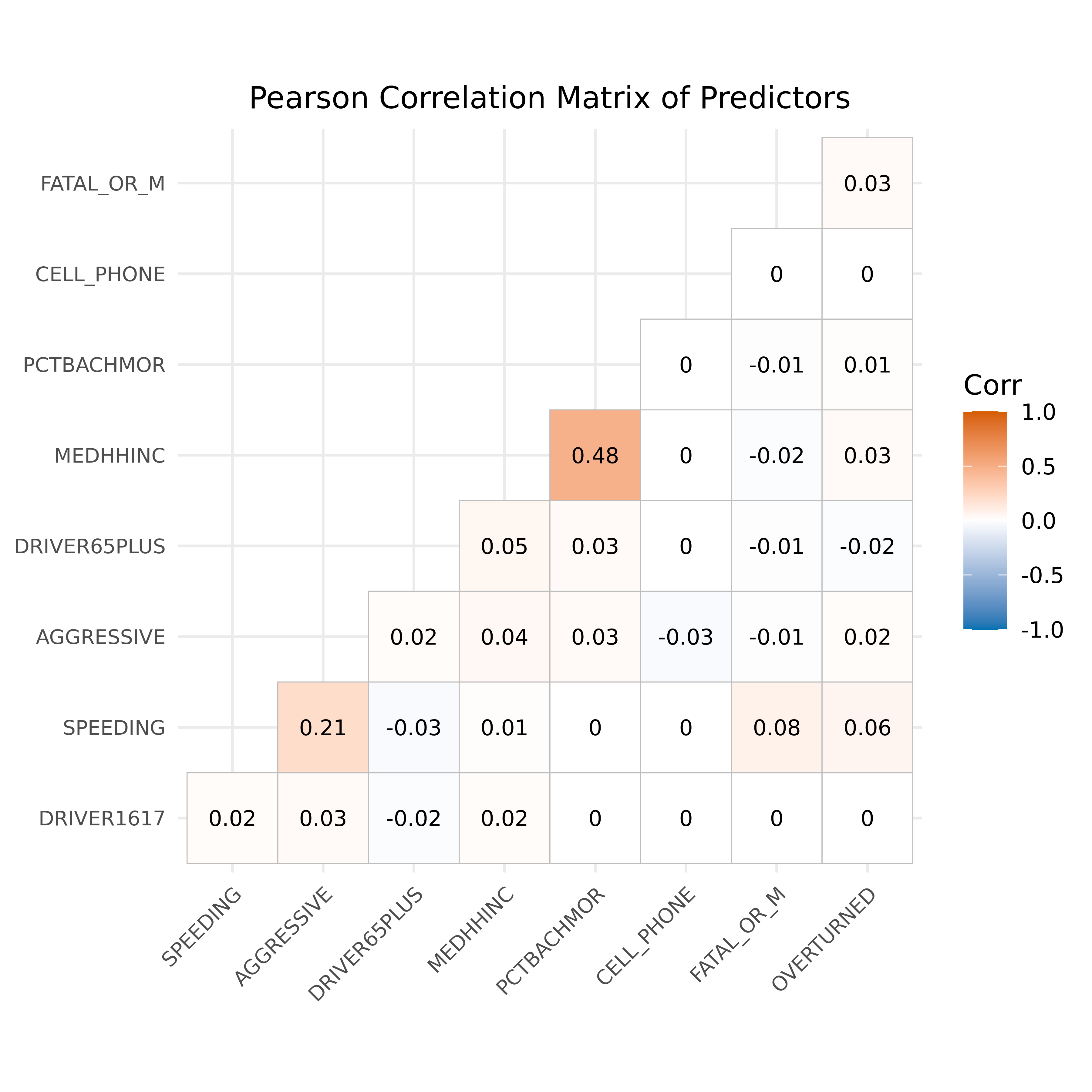
2.d. Using the instructions from Assignment 1, examine the Pearson correlations between all the predictors (both binary and continuous). Is there evidence of severe multicollinearity here? (Be sure the appropriate R library is loaded).
Warning: `aes_string()` was deprecated in ggplot2 3.0.0.
ℹ Please use tidy evaluation idioms with `aes()`.
ℹ See also `vignette("ggplot2-in-packages")` for more information.
ℹ The deprecated feature was likely used in the ggcorrplot package.
  Please report the issue at <https://github.com/kassambara/ggcorrplot/issues>.
3. Now that we’re done with exploratory analysis, we are ready to proceed to running the logistic regression.
3.a. Using the glm command for logistic regression (as shown in the slides), regress the DRINKING_D variable on the following predictors: FATAL_OR_M, OVERTURNED, CELL_PHONE, SPEEDING, AGGRESSIVE, DRIVER1617, DRIVER65PLUS, PCTBACHMOR, and MEDHHINC.
3.a.i. Use the summary command to examine the results.
full_logit_results <-cbind( full_coefs,OR = OR2,CI_low = CI2[,1],CI_high = CI2[,2])# Create table.full_model <-kbl(full_logit_results, digits =2,# Rename columns.col.names =c("Estimate", "Standard Error", "Z-Value", "P-Value", "Odds Ratio", "2.5% CI", "97.5% CI"),align ="c",caption ="Full Logistic Regression Model (Binary Predictors)") %>%kable_styling(bootstrap_options =c("striped", "hover"), full_width = F) %>%column_spec(1, bold = T) %>%footnote(general =c("<i>FATAL_OR_M:</i> Crash resulted in fatality or major injury.","<i>OVERTURNED:</i> Crash involved an overturned vehicle.","<i>CELL_PHONE:</i> Driver was using cell phone.","<i>SPEEDING:</i> Crash involved speeding car.","<i>AGGRESSIVE:</i> Crash involved aggressive driving.","<i>DRIVER1617:</i> Crash involved at least one driver who was 16 or 17 years old.","<i>DRIVER65PLUS:</i> Crash involved at least one driver who was at least 65 years old.","<i>PCTBACHMOR:</i> % of individuals 25 years of age or older who have at least a bachelor’s degree.","<i>MEDHHINC:</i> Median household income." ),general_title ="Variable Definitions:",footnote_as_chunk =FALSE, escape =FALSE# To allow HTML formatting. )# Highlight significant p-values.#row_spec(which(reduced_logit_results[, "Pr(>|z|)"] < 0.05), bold = T)full_model
Full Logistic Regression Model (Binary Predictors)
Estimate
Standard Error
Z-Value
P-Value
Odds Ratio
2.5% CI
97.5% CI
(Intercept)
-2.73
0.05
-59.56
0.00
0.07
0.06
0.07
FATAL_OR_M
0.81
0.08
9.71
0.00
2.26
1.91
2.65
OVERTURNED
0.93
0.11
8.51
0.00
2.53
2.03
3.12
CELL_PHONE
0.03
0.20
0.15
0.88
1.03
0.68
1.49
SPEEDING
1.54
0.08
19.11
0.00
4.66
3.97
5.45
AGGRESSIVE
-0.60
0.05
-12.49
0.00
0.55
0.50
0.60
DRIVER1617
-1.28
0.29
-4.37
0.00
0.28
0.15
0.47
DRIVER65PLUS
-0.77
0.10
-8.08
0.00
0.46
0.38
0.55
PCTBACHMOR
0.00
0.00
-0.29
0.77
1.00
1.00
1.00
MEDHHINC
0.00
0.00
2.09
0.04
1.00
1.00
1.00
Variable Definitions:
FATAL_OR_M: Crash resulted in fatality or major injury.
OVERTURNED: Crash involved an overturned vehicle.
CELL_PHONE: Driver was using cell phone.
SPEEDING: Crash involved speeding car.
AGGRESSIVE: Crash involved aggressive driving.
DRIVER1617: Crash involved at least one driver who was 16 or 17 years old.
DRIVER65PLUS: Crash involved at least one driver who was at least 65 years old.
PCTBACHMOR: % of individuals 25 years of age or older who have at least a bachelor’s degree.
MEDHHINC: Median household income.
Code
# Save as HTML file.#save_kable(full_model, "full_model.html", zoom = 3, self_contained = TRUE)# Then convert HTML to PNG using webshot.#webshot::webshot("full_model.html", "full_model.png")
3.a.ii. For each predictor, also compute the odds ratio and the 95% confidence interval (CI) using commands shown in the slides. Use the syntax presented on the slide titled ‘Merging Odds Ratios to 𝛽 Coefficients in R’ to merge the odds ratios and CIs to the matrix that contains coefficients and p-values. Present the resulting (merged) matrix in your report.
3.a.iii. Using the syntax presented in the slides, calculate the sensitivity, specificity and misclassification rate for each of the following cut-off values: 0.02; 0.03; 0.05; 0.07; 0.08; 0.09; 0.10; 0.15; 0.20; 0.50 and present them in a table. In the table, highlight the cut-off value which has the lowest misclassification rate.
Code
cutoffs <-c(0.02, 0.03, 0.05, 0.07, 0.08, 0.09, 0.10, 0.15, 0.20, 0.50)phat <- logit_full$fitted.valuesy <- cdc_data$DRINKING_Dcutoff_table <-data.frame(Cutoff = cutoffs,Sensitivity =NA,Specificity =NA,Misclass =NA)for (i inseq_along(cutoffs)) { c <- cutoffs[i] pred <-ifelse(phat >= c, 1, 0) TP <-sum(pred ==1& y ==1) TN <-sum(pred ==0& y ==0) FP <-sum(pred ==1& y ==0) FN <-sum(pred ==0& y ==1) cutoff_table$Sensitivity[i] <- TP/(TP+FN) cutoff_table$Specificity[i] <- TN/(TN+FP) cutoff_table$Misclass[i] <- (FP+FN)/length(y)}kable( cutoff_table,digits =3,caption ="Sensitivity, Specificity, and Misclassification Across Cutoffs")
Sensitivity, Specificity, and Misclassification Across Cutoffs
Cutoff
Sensitivity
Specificity
Misclass
0.02
0.984
0.058
0.889
0.03
0.981
0.064
0.884
0.05
0.735
0.469
0.516
0.07
0.221
0.914
0.126
0.08
0.185
0.939
0.105
0.09
0.168
0.946
0.099
0.10
0.164
0.948
0.097
0.15
0.104
0.972
0.078
0.20
0.023
0.995
0.060
0.50
0.002
1.000
0.057
: Sensitivity, Specificity, and Misclassification Table
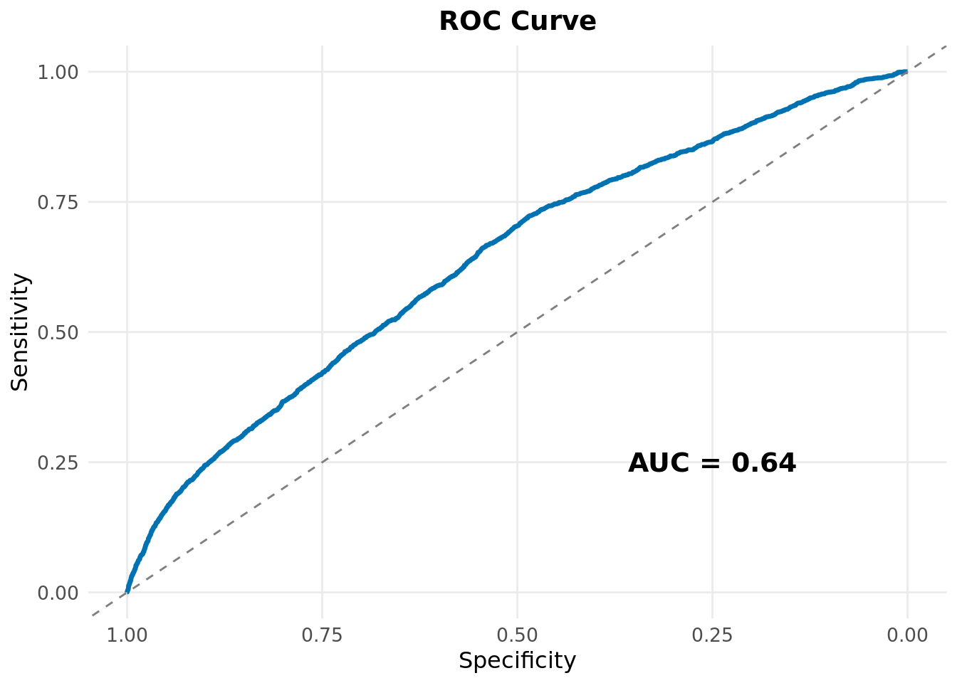
3.a.iv. Using the syntax presented in the slides, generate the ROC curve, and identify the optimal cut-off value. Be sure to export the image of the ROC curve (as you will be expected to present it in your report).
Code
library(pROC)
Type 'citation("pROC")' for a citation.
Attaching package: 'pROC'
The following object is masked from 'package:gmodels':

    ci
The following objects are masked from 'package:stats':

    cov, smooth, var
# Get AUCauc_value <-auc(roc_obj)# Plot with ggplotroc_curve <-ggroc(roc_obj, color ="#0072B2", size =1.2) +geom_abline(intercept =1, slope =1, linetype ="dashed", color ="gray50") +annotate("text", x =0.25, y =0.25, label =paste("AUC =", round(auc_value, 3)), size =5, fontface ="bold") +labs(title ="ROC Curve",x ="Specificity",y ="Sensitivity" ) +theme_minimal() +theme(plot.title =element_text(hjust =0.5, size =14, face ="bold"),axis.title =element_text(size =12),axis.text =element_text(size =10),panel.grid.minor =element_blank() )
Warning: Using `size` aesthetic for lines was deprecated in ggplot2 3.4.0.
ℹ Please use `linewidth` instead.
ℹ The deprecated feature was likely used in the pROC package.
  Please report the issue at <https://github.com/xrobin/pROC/issues>.
3.a.v. Using the syntax presented in the slides, calculate the area under the ROC curve.
3.b. Re-run the model without the PCTBACHMOR and MEDHHINC terms. As in 3.a.i and 3.a.ii above, use the summary command to examine results, and calculate the odds ratio and the 95% confidence interval for each predictor. As in 3.a.ii above, merge the odds ratios and confidence intervals to the matrix containing coefficients and p-values. Present the resulting (merged) matrix in your report.
reduced_logit_results <-cbind( reduced_coefs,OR = OR2,CI_low = CI2[,1],CI_high = CI2[,2])# Create table.reduced_model <-kbl(reduced_logit_results, digits =2,# Rename columns.col.names =c("Estimate", "Standard Error", "Z-Value", "P-Value", "Odds Ratio", "2.5% CI", "97.5% CI"),align ="c",caption ="Reduced Logistic Regression Model (Binary Predictors)") %>%kable_styling(bootstrap_options =c("striped", "hover"), full_width = F) %>%column_spec(1, bold = T) %>%footnote(general =c("<i>FATAL_OR_M:</i> Crash resulted in fatality or major injury.","<i>OVERTURNED:</i> Crash involved an overturned vehicle.","<i>CELL_PHONE:</i> Driver was using cell phone.","<i>SPEEDING:</i> Crash involved speeding car.","<i>AGGRESSIVE:</i> Crash involved aggressive driving.","<i>DRIVER1617:</i> Crash involved at least one driver who was 16 or 17 years old.","<i>DRIVER65PLUS:</i> Crash involved at least one driver who was at least 65 years old." ),general_title ="Variable Definitions:",footnote_as_chunk =FALSE, escape =FALSE# To allow HTML formatting. )# Highlight significant p-values.#row_spec(which(reduced_logit_results[, "Pr(>|z|)"] < 0.05), bold = T)# Save as HTML file.#save_kable(reduced_model, "reduced_model.html", zoom = 3, self_contained = TRUE)# Then convert HTML to PNG using webshot.#webshot::webshot("reduced_model.html", "reduced_model.png")
3.c. Compare the two models using the Akaike Information Criterion (AIC). The results are typically presented at the bottom of the logistic regression output. They may also be obtained using the AIC command. For instance, if the results obtained from the glm command for the first model are saved as mylogit1 and the results from the second model are saved as mylogit2, the R syntax to obtain the AICs from both models would be AIC(mylogit1, mylogit2). Here, recall that lower values of the AIC correspond to a better model.
# Split data into No Alcohol and Alcohol.no_alcohol <-subset(binary_summary, DRINKING_D =="No Alcohol")alcohol <-subset(binary_summary, DRINKING_D =="Alcohol")# Create a wide dataframe with one row per predictor.# Extract the counts and percents from alcohol categories.wide_summary <-data.frame(Predictor = no_alcohol$Predictor,N_No = no_alcohol$Count_1,Pct_No = no_alcohol$Percent_1,N_Yes = alcohol$Count_1,Pct_Yes = alcohol$Percent_1,Total = no_alcohol$Total_1 )# Merge with the Chi-Square P-Values.final_table_data <-merge(wide_summary, chi_results[, c("Predictor", "p_value")], by ="Predictor")# Re-order rows to match original predictor list.final_table_data <- final_table_data[match(predictors, final_table_data$Predictor), ]# Create table.cross_tab <-kbl(final_table_data, col.names =c("Predictor", "N", "%", "N", "%", "Total", "Χ2 p-value"),align =c("l", "c", "c", "c", "c", "c", "c"),digits =2,row.names =FALSE,format.args =list(big.mark =","),caption ="Cross-Tabulation of Predictors by Alcohol Involvement") %>%kable_styling(bootstrap_options =c("striped", "hover", "condensed"), full_width = F) %>%add_header_above(c(" "=1, "No Alcohol Involved\n(DRINKING_D = 0)"=2, "Alcohol Involved\n(DRINKING_D = 1)"=2, " "=2)) %>%column_spec(1, bold =TRUE) %>%footnote(general =c("<i>FATAL_OR_M:</i> Crash resulted in fatality or major injury.","<i>OVERTURNED:</i> Crash involved an overturned vehicle.","<i>CELL_PHONE:</i> Driver was using cell phone.","<i>SPEEDING:</i> Crash involved speeding car.","<i>AGGRESSIVE:</i> Crash involved aggressive driving.","<i>DRIVER1617:</i> Crash involved at least one driver who was 16 or 17 years old.","<i>DRIVER65PLUS:</i> Crash involved at least one driver who was at least 65 years old." ),general_title ="Variable Definitions:",footnote_as_chunk =FALSE, escape =FALSE# To allow HTML formatting. )cross_tab
Cross-Tabulation of Predictors by Alcohol Involvement
No Alcohol Involved
(DRINKING_D = 0)
Alcohol Involved
(DRINKING_D = 1)
Predictor
N
%
N
%
Total
Χ2 p-value
FATAL_OR_M
1,181
2.89
188
7.57
1,369
0.00
OVERTURNED
612
1.50
110
4.43
722
0.00
CELL_PHONE
426
1.04
28
1.13
454
0.69
SPEEDING
1,261
3.08
260
10.46
1,521
0.00
AGGRESSIVE
18,522
45.31
916
36.86
19,438
0.00
DRIVER1617
674
1.65
12
0.48
686
0.00
DRIVER65PLUS
4,237
10.36
119
4.79
4,356
0.00
Variable Definitions:
FATAL_OR_M: Crash resulted in fatality or major injury.
OVERTURNED: Crash involved an overturned vehicle.
CELL_PHONE: Driver was using cell phone.
SPEEDING: Crash involved speeding car.
AGGRESSIVE: Crash involved aggressive driving.
DRIVER1617: Crash involved at least one driver who was 16 or 17 years old.
DRIVER65PLUS: Crash involved at least one driver who was at least 65 years old.
Code
# Save as HTML file.#save_kable(cross_tab, "cross_tabulation_table.html", zoom = 3, self_contained = TRUE)# Then convert HTML to PNG using webshot.#webshot::webshot("cross_tabulation_table.html", "cross_tabulation_table.png")
Code
# Split the data into groups.no_alcohol_means <-subset(mean_sd_table, Group =="No Alcohol")alcohol_means <-subset(mean_sd_table, Group =="Alcohol")# Make wide.wide_means <-data.frame(Predictor = no_alcohol_means$Predictor,Mean_No = no_alcohol_means$Mean,SD_No = no_alcohol_means$SD,Mean_Yes = alcohol_means$Mean,SD_Yes = alcohol_means$SD)# Merge with t-test results to get the p-value.final_means_data <-merge(wide_means, t_table[, c("Predictor", "p_value")], by ="Predictor")# Create table.means_of_predictors <-kbl(final_means_data, col.names =c("Predictor", "Mean", "SD", "Mean", "SD", "t-test p-value"),align =c("l", "c", "c", "c", "c", "c"),digits =2,row.names =FALSE,format.args =list(big.mark =","),caption ="Means of Predictors by Alcohol Involvement") %>%kable_styling(bootstrap_options =c("striped", "hover"), full_width = F) %>%add_header_above(c(" "=1, "No Alcohol Involved\n(DRINKING_D = 0)"=2, "Alcohol Involved\n(DRINKING_D = 1)"=2, " "=1)) %>%column_spec(1, bold = T) %>%footnote(general =c("<i>PCTBACHMOR:</i> % with bachelor's degree or more.","<i>MEDHHINC:</i> Median household income." ),general_title ="Variable Definitions:",footnote_as_chunk =FALSE, escape =FALSE )means_of_predictors
Means of Predictors by Alcohol Involvement
No Alcohol Involved
(DRINKING_D = 0)
Alcohol Involved
(DRINKING_D = 1)
Predictor
Mean
SD
Mean
SD
t-test p-value
MEDHHINC
31,483.05
16,930.10
31,998.75
17,810.50
0.16
PCTBACHMOR
16.57
18.21
16.61
18.72
0.91
Variable Definitions:
PCTBACHMOR: % with bachelor's degree or more.
MEDHHINC: Median household income.
Code
# Save as HTML file.#save_kable(means_of_predictors, "means_of_predictors.html", zoom = 3, self_contained = TRUE)# Then convert HTML to PNG using webshot.#webshot::webshot("means_of_predictors.html", "means_of_predictors.png")
Code
# Find the index of the row with the minimum misclassification rate.best_row <-which.min(cutoff_table$Misclass)worst_row <-which.max(cutoff_table$Misclass)cutoff_table <-kbl(cutoff_table, digits =2,caption ="Sensitivity, Specificity, and Misclassification Rates") %>%kable_styling(bootstrap_options =c("striped", "hover"), full_width = F) %>%# Bold best row.row_spec(best_row, bold =TRUE, color ="black") %>%# Bold worst row.row_spec(worst_row, bold =TRUE, color ="black")cutoff_table
Sensitivity, Specificity, and Misclassification Rates
Cutoff
Sensitivity
Specificity
Misclass
0.02
0.98
0.06
0.89
0.03
0.98
0.06
0.88
0.05
0.73
0.47
0.52
0.07
0.22
0.91
0.13
0.08
0.18
0.94
0.10
0.09
0.17
0.95
0.10
0.10
0.16
0.95
0.10
0.15
0.10
0.97
0.08
0.20
0.02
1.00
0.06
0.50
0.00
1.00
0.06
Code
# Save as HTML file.#save_kable(cutoff_table, "cutoff_table.html", zoom = 3, self_contained = TRUE)# Then convert HTML to PNG using webshot.#webshot::webshot("cutoff_table.html", "cutoff_table.png")
Code
# Calculate AIC for both modelsaic_values <-AIC(logit_full, logit_reduced)# The AIC() function returns a dataframe with row names as the models.# Let's pretty it up for the table.aic_table <-data.frame(Model =c("Full Model (All Predictors)", "Reduced Model (Binary Only)"),df = aic_values$df,AIC = aic_values$AIC)aic_kable <-kbl(aic_table, digits =2,col.names =c("Model", "Degrees of Freedom", "AIC"),align =c("l", "c", "c"),caption ="Model Comparison: Akaike Information Criterion (AIC)") %>%kable_styling(bootstrap_options =c("striped", "hover"), full_width = F) %>%row_spec(which.min(aic_table$AIC), bold = T, color ="black") %>%footnote(general =c("Lower AIC is better." ),general_title ="Note:",footnote_as_chunk =FALSE, escape =FALSE )aic_kable
Model Comparison: Akaike Information Criterion (AIC)
Model
Degrees of Freedom
AIC
Full Model (All Predictors)
10
18359.63
Reduced Model (Binary Only)
8
18360.47
Note:
Lower AIC is better.
Code
# Save as HTML file.#save_kable(aic_kable, "aic_kable.html", zoom = 3, self_contained = TRUE)# Then convert HTML to PNG using webshot.#webshot::webshot("aic_kable.html", "aic_kable.png")